The index to the articles in this series is found here.

UPDATE #1 (2019-09-02): These results are invalid due to an error in the input. We will return to this later.

I’ve done some analysis in TensorBoard, trying to find places where it looks like a layer could use some regularization. Now I present the histograms.

I start with the output from the input layer. This is just an echo of our inputs.

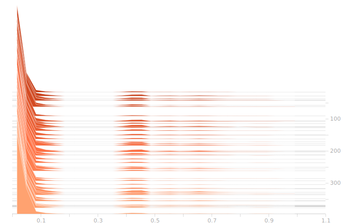
So, as we see, there are a lot of zeroes corresponding to sectors with no rain falling. Then there are peaks further out representing different intensities of rain. The large gap between the low and high rain intensities is engineered into the data, I deliberately left a wide space in the normalization so that the network could more easily distinguish light rain from heavy rain.

Next, we come to the LSTM layer.

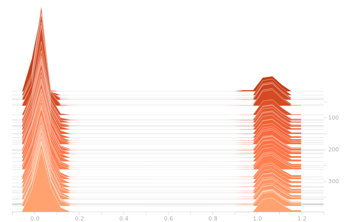
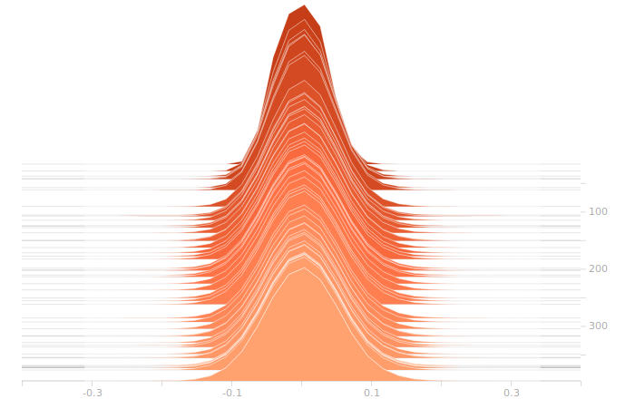
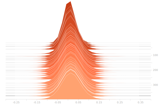
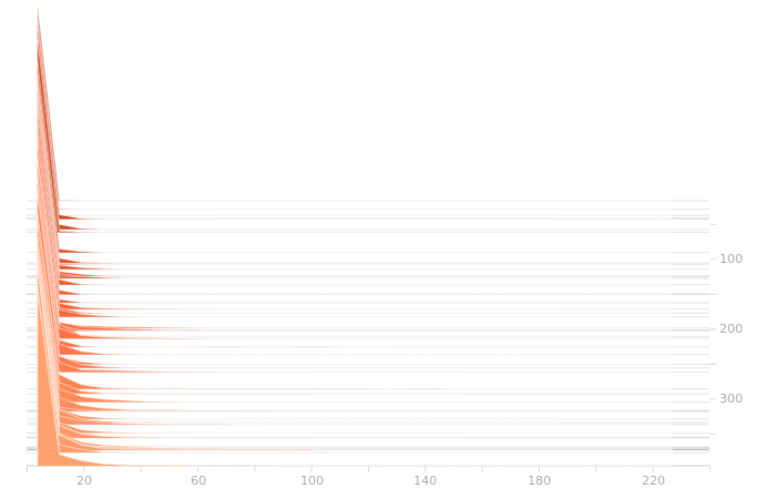
The LSTM layer is the first to encounter the input data. There’s a large block of biases at zero, and then more around 1.05. The zero biases are due to the fact that a large number of sectors in the input don’t contribute to the outputs, and so aren’t seeing training. This is because our training set doesn’t have rain coming from arbitrary directions, it’s all coming from approximately WSW to approximately ENE. The output bits do not depend on rain East of Ottawa, because that rain is moving away, not moving toward us. The relative size of those regions just shows what fraction of the disc centred on Franktown can be responsible for rain in Ottawa.

There isn’t really any more interesting structure in the weights. This is a bit disappointing, I was hoping for a clear sign of some weights becoming overbalanced, but that doesn’t seem to be the case.

On to the synthesis layer:

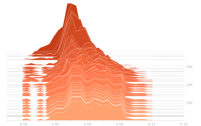
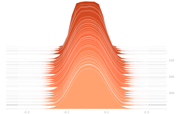
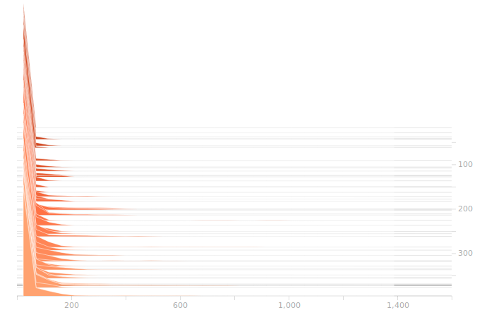
Once again, I don’t see anything suggestive of overbalanced weights. The synthesis layer is starting to show multimodal distributions in the biases, this is due to the fact that we’ve got to inform 10 separate bits in the output. The output layer will show this even more clearly.

So, here’s the output layer:

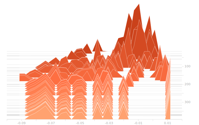
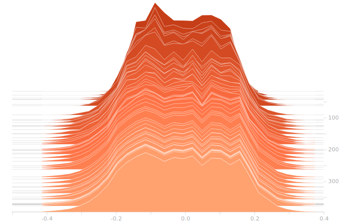
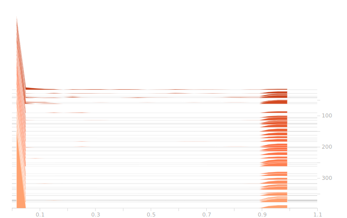
The output layer has a clear multimodal distribution of biases, which will be feeding different bits in the output. There is nothing of exceptional note in the kernel weights. The output layer outputs are strongly clustered at 0 and 1, as we would expect for a trained binary output. There is little room for ambiguity here, adjusting the threshold for declaring a value to be 0 or 1 would have negligible effect on the output of the model.

So, where do we go now? We have models that overfit eventually, but that will always happen. It’s not difficult to keep a copy of the network that produced the best validation loss, and that’s what I’ve been doing to see the results on the holdout data. We don’t have evidence that the overfitting is due to the network entering a pathological state, it seems to be operating quite nicely in the general analysis case all the way up to the point where it smoothly starts overfitting. Regularization seems unlikely to have much effect on this network.

I kind of wanted to try out some regularizations, so I’ll be testing a few, just to see the impact, after we play a bit with the network size.

One thing we see from these histograms is that the network is really not straining to produce our answers. Strong peaks, no intermediate values, this suggests that our network is bigger than it has to be. I’m going to start cutting back the size of the network to see how that changes things.