I broke my data. I was running a Knuth shuffle manually on the numpy arrays for input and true values. Apparently the familiar mechanism of TMP=A; A=B; B=TMP; doesn’t work as expected with numpy arrays and sub-arrays, and I wound up losing big swaths of data and replacing them with duplicates. I’ve corrected that, but it invalidates the results of my earlier experiments. I’ve updated earlier articles appropriately.
Tag Archives: rain predictor
Building a Rain Predictor. Analysis of weights.
The index to the articles in this series is found here.
UPDATE #1 (2019-09-02): These results are invalid due to an error in the input. We will return to this later.
I’ve done some analysis in TensorBoard, trying to find places where it looks like a layer could use some regularization. Now I present the histograms.
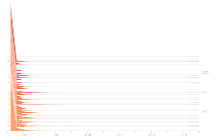
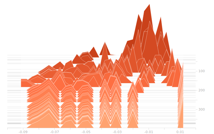
I start with the output from the input layer. This is just an echo of our inputs.
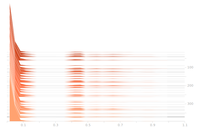
So, as we see, there are a lot of zeroes corresponding to sectors with no rain falling. Then there are peaks further out representing different intensities of rain. The large gap between the low and high rain intensities is engineered into the data, I deliberately left a wide space in the normalization so that the network could more easily distinguish light rain from heavy rain.
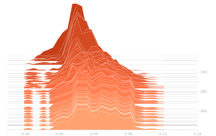
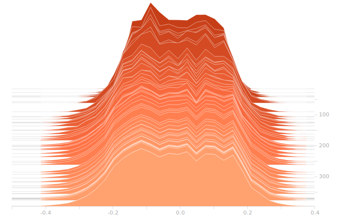
Next, we come to the LSTM layer.
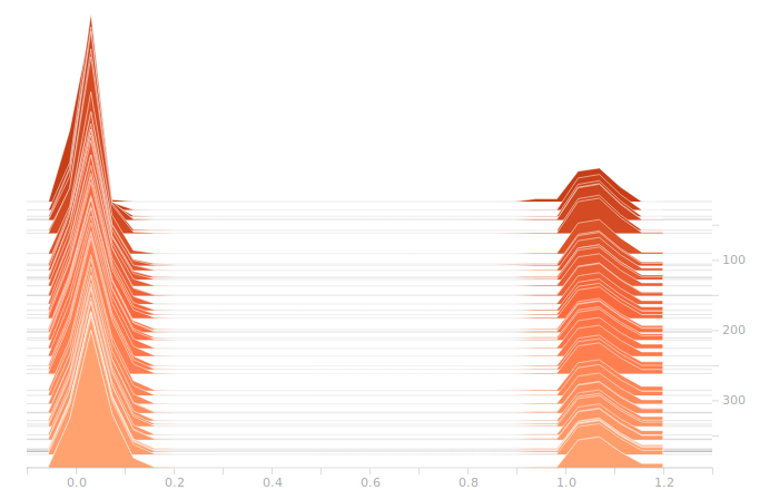
The LSTM layer is the first to encounter the input data. There’s a large block of biases at zero, and then more around 1.05. The zero biases are due to the fact that a large number of sectors in the input don’t contribute to the outputs, and so aren’t seeing training. This is because our training set doesn’t have rain coming from arbitrary directions, it’s all coming from approximately WSW to approximately ENE. The output bits do not depend on rain East of Ottawa, because that rain is moving away, not moving toward us. The relative size of those regions just shows what fraction of the disc centred on Franktown can be responsible for rain in Ottawa.
There isn’t really any more interesting structure in the weights. This is a bit disappointing, I was hoping for a clear sign of some weights becoming overbalanced, but that doesn’t seem to be the case.
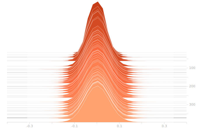
On to the synthesis layer:
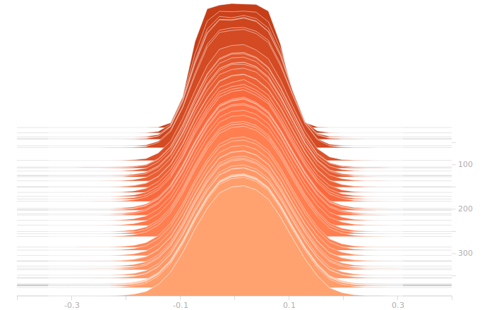
Once again, I don’t see anything suggestive of overbalanced weights. The synthesis layer is starting to show multimodal distributions in the biases, this is due to the fact that we’ve got to inform 10 separate bits in the output. The output layer will show this even more clearly.
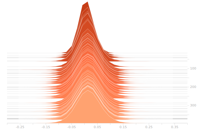
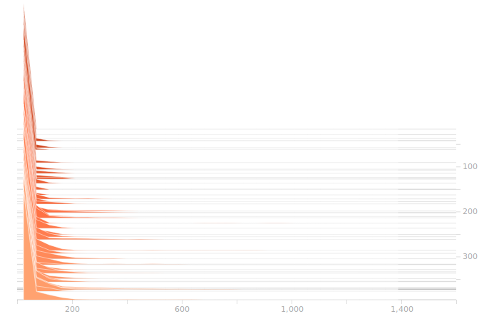
So, here’s the output layer:
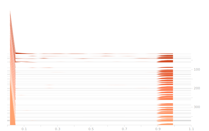
The output layer has a clear multimodal distribution of biases, which will be feeding different bits in the output. There is nothing of exceptional note in the kernel weights. The output layer outputs are strongly clustered at 0 and 1, as we would expect for a trained binary output. There is little room for ambiguity here, adjusting the threshold for declaring a value to be 0 or 1 would have negligible effect on the output of the model.
So, where do we go now? We have models that overfit eventually, but that will always happen. It’s not difficult to keep a copy of the network that produced the best validation loss, and that’s what I’ve been doing to see the results on the holdout data. We don’t have evidence that the overfitting is due to the network entering a pathological state, it seems to be operating quite nicely in the general analysis case all the way up to the point where it smoothly starts overfitting. Regularization seems unlikely to have much effect on this network.
I kind of wanted to try out some regularizations, so I’ll be testing a few, just to see the impact, after we play a bit with the network size.
One thing we see from these histograms is that the network is really not straining to produce our answers. Strong peaks, no intermediate values, this suggests that our network is bigger than it has to be. I’m going to start cutting back the size of the network to see how that changes things.
Building a Rain Predictor. Regularizing the weights.
The index to the articles in this series is found here.
UPDATE #1 (2019-09-02): These results are invalid due to an error in the input. We will return to this later.
So, regularizing. This is a technique used to address overfitting. We’ve discussed overfitting before. One possible approach is to reduce the dimensionality of the network, use fewer neurons. Another is to find a way to penalize undesirable weight configurations so that the network is more likely to find a general solution, rather than a specific fit to the training data.
We’re going to explore some different approaches. One is a direct weight penalty, the other is a dropout layer. The dropout layer randomly zeroes a certain fraction of the inputs to the following layer. The effect of this is to penalize network configurations that depend too much on a specific small set of correlated inputs, while almost ignoring all the other inputs. Such an undesirable configuration would produce large losses when the dropout layer removed some of its inputs, allowing the network to train to a more resilient configuration that is less dependent on a narrow subset of its inputs.
The direct weight penalty is fairly obvious, the training loss is increased by the presence of large weights, thereby training the network toward weights of a more uniform distribution. There are two typical metrics used for minimization, referred to as L1 and L2. In L1 regularization, also referred to as Lasso regression, a term proportional to the absolute values of the weights is added to the loss function. In L2, or Ridge regression, a term proportional to the square of the weights is added. Each regularization technique also includes a free parameter, the proportionality constant for adding in the penalty, and the choice of this number can have an important impact on the quality of the final model.
To begin, we’re going to re-run our optimizers, with batch sizes of 512 now, and train out 400 epochs. At the end of that time, we will generate a histogram of the weights in the different layers, to see which layers, if any, have a badly unbalanced weight distribution. These will be candidates for our regularization techniques, either through one of Lasso or Ridge regression, or with a dropout layer.
I will not be using a dropout layer on the LSTM layer, since its inputs are often dominated by zeroes, only a relatively small fraction of the input data is non-zero. It sometimes makes sense to apply dropout to the inputs of a network, but it’s usually not useful on data of the type we have here, where the interesting feature of the data is a binary state, raining or not raining in that sector.
Recurrent layers, of which LSTM is a type, are particularly susceptible to overtraining issues with unbalanced weights, so we will be looking for problems in that layer and addressing them with regularization settings in the layer construction.
Another regularization technique that is sometimes applied is a noise layer. Random perturbations of the inputs to a layer can help the network to generalize from a specific set of values by training it to recognize as equivalent inputs that are close together in phase space. I’m not currently planning to use noise injection, we’ll see how the other approaches perform first.
In order to generate through-time histograms of weights, I’ll be using TensorBoard. To that end, I’ve modified the code in rptrainer2.py to log suitable data. The output files are huge, but I hope to get some useful information from them.
Building a Rain Predictor. Results of first experiments
The index to the articles in this series is found here.
UPDATE #1 (2019-09-02): These results turn out to be invalid. I was doing a Knuth shuffle on rows in a numpy array for the inputs and true values, and apparently there are subtleties in swapping rows through a temporary value that I wasn’t aware of, because I wound up with duplicated entries (and corresponding disappearance of unique entries). I have to re-run now that I’ve fixed the shuffling code.
I’ve run through all of the optimizers bundled with Keras. Originally, I had been tracking CPU time, but I stopped. First of all, execution time was very similar in all experiments, roughly 2 wallclock hours to run 400 epochs. Secondly, for all experiments after the first, the best network wasn’t the one at epoch 400, but an earlier, sometimes much earlier one, before the network began to overtrain and the validation data loss worsened.
I decided that, for these experiments, I’d focus on one particular result in the holdout data. If it is currently not raining, and will start raining in more than 1 hour but less than 2, then the network will be considered to have a successful prediction if it predicts rain any time in the next 2 hours. I’ll call this the “one hour warning” success rate.
Here are the results from the first run of experiments:
| Experiment | Training Loss | Validation Loss | One Hour Warning Rate |
| SGD | 0.0638 | 0.0666 | 0.56 |
| RMSProp default | 0.0247 | 0.0383 | 0.88 |
| RMSProp large batch | 0.0074 | 0.0102 | 0.96 |
| RMSProp Small LR | 0.0180 | 0.0293 | 0.84 |
| Adagrad | 0.0018 | 0.0111 | 0.93 |
| Adadelta | 0.0102 | 0.0186 | 0.91 |
| Adam | 0.0066 | 0.0102 | 0.83 |
| Adamax | 0.0026 | 0.0069 | 0.84 |
| Nadam | 0.0090 | 0.0228 | 0.78 |
So, do we just declare that RMSProp large batch is the best result and continue? Well, no, we can’t do that. First, we know that the large batch size improves RMSProp, and we didn’t test a large batch size on the other optimizers. Second, we have to compute statistics on our one-hour warning rate. For RMSProp large batch, the uncertainty in the result is 0.027 at the 90% confidence level using the student T-test. This is, in fact, a lower bound on the uncertainty. There are 146 eligible samples that match the requirements for a one-hour warning test, but these aren’t strictly independent. Many of these might just be the same rain event but with the historical window starting 10 or 20 minutes later, so a significant fraction of the input time steps is shared between so-called independent measurements.
All right, so we know, on broad arguments, that a larger batch size is really required for any of these tests in this particular project. We’ll have to re-run with a larger batch size. We’ll also want to start putting in regularizers. From now on, all our experiments will be made with a batch size of 512, unless otherwise noted. The larger batch size will reduce the amount of convergence we achieve per epoch, but the epochs are also 4 times faster, so we don’t expect any great increase in runtime.
In the next post, we’ll begin the regularizer testing.
Building a Rain Predictor. Another optimizer.
The index to the articles in this series is found here.
OK, I’m not going to turn this series of posts into a stack of plots of loss vs. epoch number, that’s not why we’re here. There is, however, one more I’d like to show. In the last post we saw some training results that were strongly suggestive of overfitting. I’m going to show one here that is unambiguous. This is the Adagrad optimizer in Keras, with default settings and batch size. This optimizer is a good choice for fitting sparse data. Even after thinning our dataset to remove many uninteresting inputs, any particular bit in the output set is still fairly sparse, so this seems a promising candidate.
Plotting the losses against epoch number again, we see this:
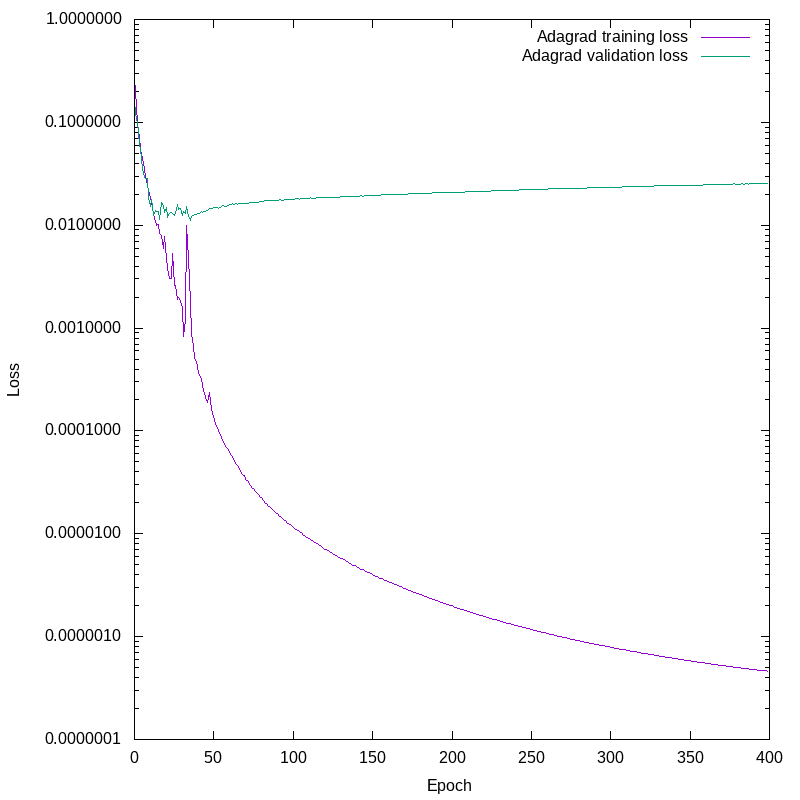
This is unambiguous. Note the logarithmic scale on the Y axis. Fairly early on, the validation loss detaches from the training loss. The network continues to improve the training loss by four decades, while the validation loss slowly increases. From about epoch 20 onward we are not improving the network’s ability to predict the future given new data, we are only getting it more and more obsessively correct about the training set, and our predictions on novel data are worsening.
All right, I’ve got four more optmizers bundled with Keras to test. I won’t post about those in detail unless something new appears, interesting in a different way. Once I’ve run through all the optimizers, I’ll present some other data about how well the resulting networks performed.