The index to the articles in this series is found here.
With a few tweaks to the phantom rain detection, suddenly things are looking much better. My two hour warning time is now 0.83, and the failed predictions are difficult cases. Examining the predictions that failed shows rain that forms directly overhead, with no warning on radar, or small rain pockets that could either pass by the city or pass overhead. They’re cases that I wouldn’t be able to predict better by looking at the same images. So, that’s a success. I can feed a set of radar images into the neural network and have it tell me whether or not to expect rain.
What’s left to do? Now we can still experiment a bit to see if we can find a way to reduce the fraction of failed predictions. Ideally we want incorrect predictions to have lower confidence than successful ones. By histogramming the (floating point) predicted values for successful and failed predictions, I hope I can come up with a confidence level. A value of less than 0.02 indicates a firm prediction of false. A value of greater than 0.98 indicates a firm prediction of true. In between, we have lower confidence warnings. There’s a cutoff at 0.5 between predicting positive or negative results. Shifting that cutoff has the effect of trading false negative for false positives, or vice versa. I’m not going to focus on this, though.
So, I’m going to try to play around with network settings now to see if I can separate the false positives from true positives, and conversely for negatives. Right now, there’s a handful of false negatives with a value less than 0.02, which indicates a firm false prediction. I’d like to train a network that minimizes those high confidence incorrect predictions.
Postings will probably slow down a bit now, as I experiment with settings and see how changes behave.
In the mean time, I’m happy with the results of this project.
The index to the articles in this series is found here.
I’ve now re-run the experiments over 200 epochs. In the first set of runs, the overfitting manifested fairly early, within 100 epochs, so I didn’t see a need to run out to 400 epochs this time. The SGD optimizer is still working at 200 (and was still working at 400 in earlier tests). The other optimizers have long since established their networks.
Experiment
Training Loss
Validation Loss
Two Hour Warning
SGD
0.3135
0.3057
0.00
RMSProp
0.0480
0.0796
0.82
Adagrad
0.0317
0.0823
0.78
Adadelta
0.0733
0.0829
0.77
Adam
0.0300
0.0872
0.77
Adamax
0.0340
0.1148
0.81
Nadam
0.0789
0.0929
0.80
Examining the loss numbers, it turns out that Adadelta hadn’t reached overfitting yet, and was still improving against the validation set, so I re-ran that one with 400 epochs, and it settled at a two hour warning fraction of 0.82.
One thing we see in this table is that there’s really no great difference, from a final model accuracy standpoint, between the various optimizers. Excluding the SGD, which would probably get there eventually if I let it run long enough, the other optimizers arrive at similarly accurate solutions. They differ in how quickly they arrive there, and as we saw in an earlier posting, some can diverge if the batch size is too small and the training is performed on batches that are not statistically similar to the overall population. Otherwise, I can limit my experimentation to a single optimizer, at least for a while. I might, at the end, re-run tests with all optimizers to see if any interesting differences in performance have been teased out by whatever configuration changes I make. I’ll be using the RMSprop optimizer for the next while, unless otherwise explicitly noted.
These numbers are disappointing, I liked it when they were at 0.96. Let’s analyse why the corrupted data did so much better, because it helps to emphasize why it’s critically important to have separate datasets for training and validation.
So, the problem occurred because I was manually shuffling two numpy arrays in parallel, using a Knuth shuffle. In this shuffling algorithm, we loop from the first element of the array to one before the last. At each element, we choose a random element between the element itself and the final element in the array, and swap this element with that other one. We never revisit earlier elements, and the random choice includes the same element, so there’s a chance that the element swaps with itself. It is easy to prove that in the final shuffled state, each element has an equal probability of being placed in each slot, so we have a true, fair shuffle.
I was swapping with the familiar mechanism: TMP = A; A = B; B = TMP. It appears, however, that the assignment to temporary space is a pointer, not a deep copy. So, modifying A also modifies TMP. This means that after the swap is complete, B appears twice, and A has disappeared. That assignment is a deep copy, if B is changed, A doesn’t change in sympathy.
Now, I was using Keras’ facility for splitting data into training and validation. This is done by taking a certain number of elements off the end of the input array before Keras does its own shuffling for purposes of splitting into batches.
We can analyse the effect of our broken shuffling on the distribution of elements, and, in particular, find out how many elements from the last 20% of the array wind up in the first 80% where the training will see them. Note that, because elements only move back in the array, training data never gets into the validation data, but validation data can wind up in the training data.
The probability that the first element in the training set will be copied from the validation data is
P_{1} = \frac{V}{N_{tot}}
where V is the number of elements in the validation segment, and N_{tot} is the total number of elements.
The probability that the second element will be copied from the validation data is
P_{2} = \frac{V}{N_{tot} - 1}
The expected number of validation elements that appear in the training data is, then
<N_{V}> = \sum_{k=0}^{N-V-1} \frac{V}{N - k}
This is just a bit of arithmetic on harmonic numbers.
<N_{V}> = V [ H_{N} - H_{N - k}]
This simplifies to:
<N_{V}> = V [ ln(N) - ln(N-k) + \mathcal{O}(\frac{k}{N(N-k)})]
When k is 20% of N, and N is in the thousands, as in our case, about 22% of the training set actually contains validation data.
So, unless your network has too few degrees of freedom to describe the problem, or is exactly balanced, then, barring convergence pathologies, you will eventually overfit the model. If your training data contains a significant fraction of your validation data, then you will appear to be doing very well on validation, because you trained against it.
What about the probability that any specific element in the validation set has not accidentally been placed in the training set? This is the product of the probabilities for each element in the training set:
Therefore, we expect 80% of our validation elements to be present in the training set, some duplicated, and 22% of our training set to contain validation elements. And that completely messes up our statistics, making it look like our network was doing much better than it truly was.
Where do we go from here? First, let’s look at the nature of a failing prediction. I pull one failure out and look at the historical rainfall, then the rain starting two hours later.
Historical data feeding network“Future” data feeding true Y vals 2 hours later
Yeah, there’s no rain there. What’s going on? The network got the correct answer, it’s the training “true” values that are wrong. You recall I had to deal with what I called “phantom rain”. That’s the scattering of light rain points around the radar station. Not really rain, it seems to be related to close range scattering from humid air. I don’t see a mention of this style of false image on Environment Canada’s page detailing common interpretation errors. I decided to use a rule that said that this false rain is declared to be occurring when only the lowest intensity of rain is seen within a certain radius of the radar station, and those rain pixels make up less than 50% of the area of the disc. Well, in the image that declares that there is rain in Ottawa at that particular time, there is a single phantom rain pixel of intensity 2, South-East of the station. This is enough for the data generation system to declare that another phantom rain pixel over Ottawa is real rain, and the training data gets an incorrect Y value. I brought up another image from a failed prediction, and there was a single pixel of intensity 3, North-North-West of the station.
All right, so my data cleaning operation didn’t work as well as it should have. Neural networks are notoriously sensitive to dirty data, as they work hard to imagine some sort of correlation between events that didn’t actually take place.
Recall that all of our networks overtrained, and based on the values of the training losses, reproduced their inputs essentially exactly when subject to a 0.5 mid-point decision cutoff between rain and no-rain. That means that our overtrained networks actually managed to declare those phantom rain pixels as rain, when they should not have done so. The best matching networks, though, the ones with the lowest validation losses, correctly indicated that there was no rain in those images, and we scored them lower because they failed to match the incorrect Y values. Validation loss doesn’t feed back into the network weights during training, so the network didn’t force itself to give wrong answers on these entries.
That’s actually very encouraging. Now all we have to do is to figure out how to identify phantom rain more accurately, regenerate our Y values, and try again. Well, I have a nice list of 30 or so bad cases, taken from the holdout data set. The neural network has helpfully presented me with a good set of incorrectly-classified images that I can use to improve my data cleaning efforts.
So, let’s not say we need exactly zero pixels of higher intensity than the lowest for the rain to be declared phantom rain. Instead, we’ll say that as long as there are fewer than 5 such pixels, there’s still a possibility of phantom rain. That’s an edit to prepare-true-vals.py.
I broke my data. I was running a Knuth shuffle manually on the numpy arrays for input and true values. Apparently the familiar mechanism of TMP=A; A=B; B=TMP; doesn’t work as expected with numpy arrays and sub-arrays, and I wound up losing big swaths of data and replacing them with duplicates. I’ve corrected that, but it invalidates the results of my earlier experiments. I’ve updated earlier articles appropriately.
The index to the articles in this series is found here.
UPDATE #1 (2019-09-02): These results are invalid due to an error in the input. We will return to this later.
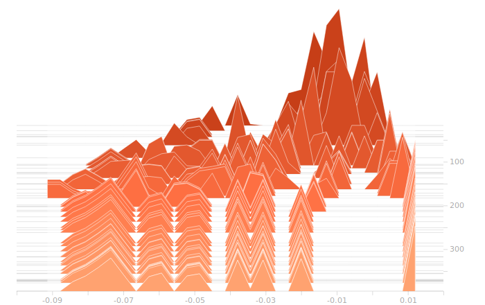
I’ve done some analysis in TensorBoard, trying to find places where it looks like a layer could use some regularization. Now I present the histograms.
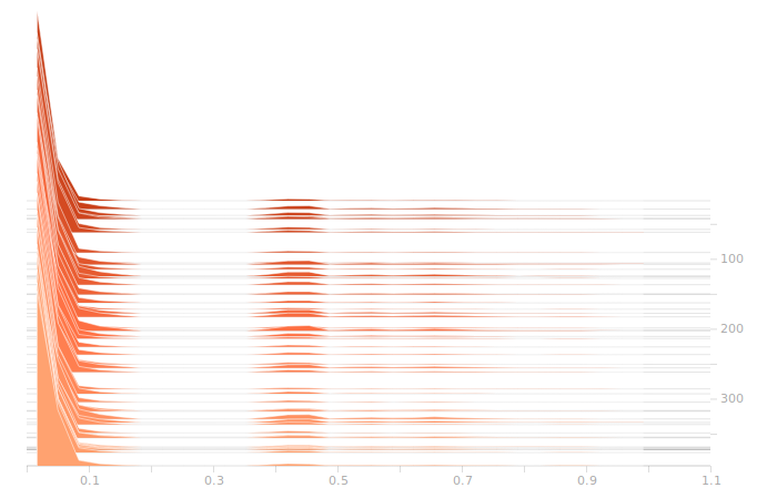
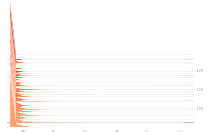
I start with the output from the input layer. This is just an echo of our inputs.
The input layer’s output
So, as we see, there are a lot of zeroes corresponding to sectors with no rain falling. Then there are peaks further out representing different intensities of rain. The large gap between the low and high rain intensities is engineered into the data, I deliberately left a wide space in the normalization so that the network could more easily distinguish light rain from heavy rain.
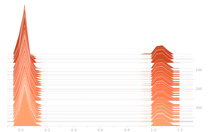
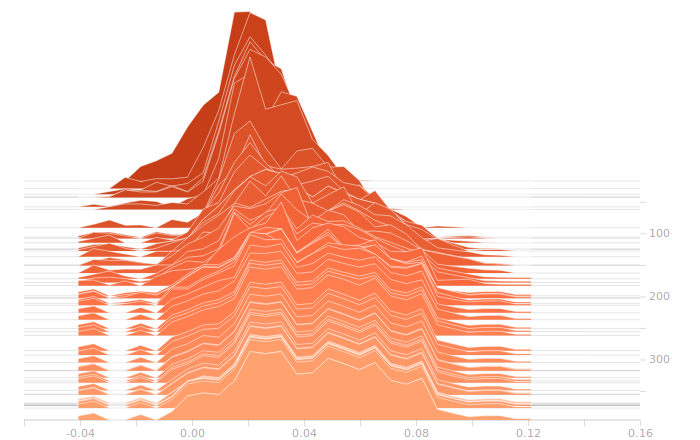
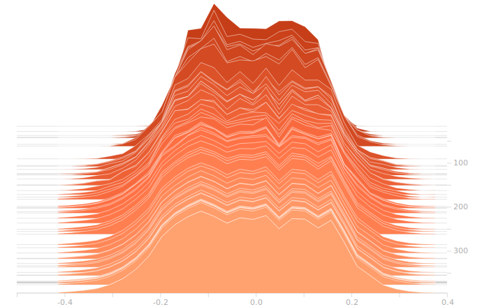
The LSTM layer is the first to encounter the input data. There’s a large block of biases at zero, and then more around 1.05. The zero biases are due to the fact that a large number of sectors in the input don’t contribute to the outputs, and so aren’t seeing training. This is because our training set doesn’t have rain coming from arbitrary directions, it’s all coming from approximately WSW to approximately ENE. The output bits do not depend on rain East of Ottawa, because that rain is moving away, not moving toward us. The relative size of those regions just shows what fraction of the disc centred on Franktown can be responsible for rain in Ottawa.
There isn’t really any more interesting structure in the weights. This is a bit disappointing, I was hoping for a clear sign of some weights becoming overbalanced, but that doesn’t seem to be the case.
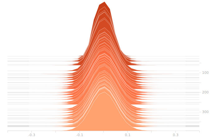
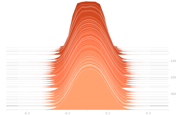
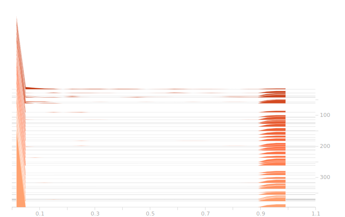
Once again, I don’t see anything suggestive of overbalanced weights. The synthesis layer is starting to show multimodal distributions in the biases, this is due to the fact that we’ve got to inform 10 separate bits in the output. The output layer will show this even more clearly.
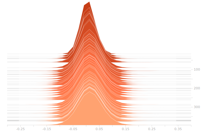
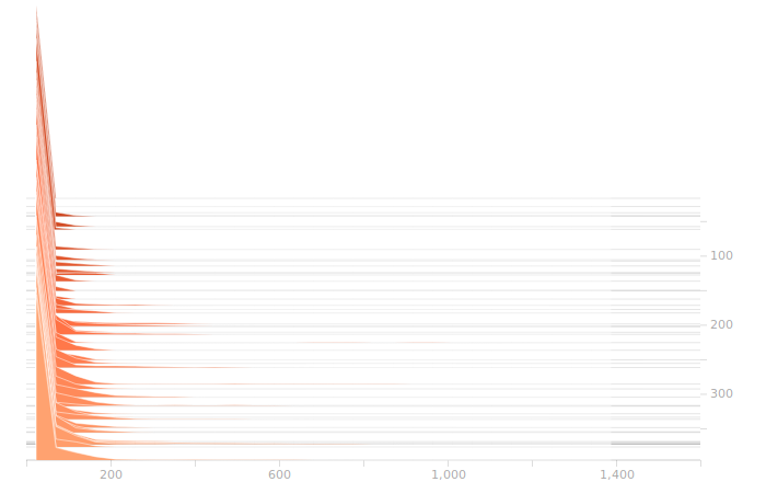
The output layer has a clear multimodal distribution of biases, which will be feeding different bits in the output. There is nothing of exceptional note in the kernel weights. The output layer outputs are strongly clustered at 0 and 1, as we would expect for a trained binary output. There is little room for ambiguity here, adjusting the threshold for declaring a value to be 0 or 1 would have negligible effect on the output of the model.
So, where do we go now? We have models that overfit eventually, but that will always happen. It’s not difficult to keep a copy of the network that produced the best validation loss, and that’s what I’ve been doing to see the results on the holdout data. We don’t have evidence that the overfitting is due to the network entering a pathological state, it seems to be operating quite nicely in the general analysis case all the way up to the point where it smoothly starts overfitting. Regularization seems unlikely to have much effect on this network.
I kind of wanted to try out some regularizations, so I’ll be testing a few, just to see the impact, after we play a bit with the network size.
One thing we see from these histograms is that the network is really not straining to produce our answers. Strong peaks, no intermediate values, this suggests that our network is bigger than it has to be. I’m going to start cutting back the size of the network to see how that changes things.
The index to the articles in this series is found here.
UPDATE #1 (2019-09-02): These results are invalid due to an error in the input. We will return to this later.
So, regularizing. This is a technique used to address overfitting. We’ve discussed overfitting before. One possible approach is to reduce the dimensionality of the network, use fewer neurons. Another is to find a way to penalize undesirable weight configurations so that the network is more likely to find a general solution, rather than a specific fit to the training data.
We’re going to explore some different approaches. One is a direct weight penalty, the other is a dropout layer. The dropout layer randomly zeroes a certain fraction of the inputs to the following layer. The effect of this is to penalize network configurations that depend too much on a specific small set of correlated inputs, while almost ignoring all the other inputs. Such an undesirable configuration would produce large losses when the dropout layer removed some of its inputs, allowing the network to train to a more resilient configuration that is less dependent on a narrow subset of its inputs.
The direct weight penalty is fairly obvious, the training loss is increased by the presence of large weights, thereby training the network toward weights of a more uniform distribution. There are two typical metrics used for minimization, referred to as L1 and L2. In L1 regularization, also referred to as Lasso regression, a term proportional to the absolute values of the weights is added to the loss function. In L2, or Ridge regression, a term proportional to the square of the weights is added. Each regularization technique also includes a free parameter, the proportionality constant for adding in the penalty, and the choice of this number can have an important impact on the quality of the final model.
To begin, we’re going to re-run our optimizers, with batch sizes of 512 now, and train out 400 epochs. At the end of that time, we will generate a histogram of the weights in the different layers, to see which layers, if any, have a badly unbalanced weight distribution. These will be candidates for our regularization techniques, either through one of Lasso or Ridge regression, or with a dropout layer.
I will not be using a dropout layer on the LSTM layer, since its inputs are often dominated by zeroes, only a relatively small fraction of the input data is non-zero. It sometimes makes sense to apply dropout to the inputs of a network, but it’s usually not useful on data of the type we have here, where the interesting feature of the data is a binary state, raining or not raining in that sector.
Recurrent layers, of which LSTM is a type, are particularly susceptible to overtraining issues with unbalanced weights, so we will be looking for problems in that layer and addressing them with regularization settings in the layer construction.
Another regularization technique that is sometimes applied is a noise layer. Random perturbations of the inputs to a layer can help the network to generalize from a specific set of values by training it to recognize as equivalent inputs that are close together in phase space. I’m not currently planning to use noise injection, we’ll see how the other approaches perform first.
In order to generate through-time histograms of weights, I’ll be using TensorBoard. To that end, I’ve modified the code in rptrainer2.py to log suitable data. The output files are huge, but I hope to get some useful information from them.