The index to the articles in this series is found here.

I got my larger data set, almost 5 years of radar data. This took about 40 hours on all cores of my home machine to convert into the intermediate binary format, but then I was able to start experimenting.

I mentioned in the last article that I had been a bit concerned about the overlapping in time of the training, validation, and holdout sets. Since I only had a handful of months of data, and rain only happens a few times a week, I decided that this was how I would break up my data set. With the new multi-year dataset, though, I could make truly independent training, validation, and holdout sets, from separate years.

And… it turns out I was right to be concerned about that overlap. With the disjoint data sets, the network can be seen to be almost immediately overtraining. That is, it is not getting any better at predicting the outcome from new data, it’s getting worse. Typically, this results in a prediction success rate of about 60% now.

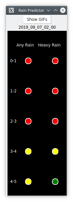
Of course, the desktop widget that I have been using has shown its usefulness, even though it was trained and validated on overlapping data. This means that that network was overtrained, and probably doing more poorly in the predictions I was using it for.

So, how do we address the overtraining? I’ve changed the geometry somewhat to start with. Now, instead of feeding the data into the LSTM layer, I first feed it into a geometry layer that takes the 800+ inputs and produces a smaller number of outputs to feed into the LSTM layer. I apply batch normalization to that layer, and a 50% dropout, before going on to LSTM. After LSTM, another 50% dropout, then into another normalized dense layer, then finally the output layer. I cut way back on the sizes of my layers, instead of hundreds of nodes per layer, I’m down to tens.

Even with all that, the network overtrains immediately. I have to find a better way to design the network to capture generic features, rather than specific details.

Early on, when the scope of the problem became apparent, I said I was not going to use convolutional layers. The size of the data appeared to make that impractical. I’m now going back and thinking about that decision. I have some ideas for how I can apply convolutions without straining the memory of the machine. I was thinking of doing it in polar coordinates, the way the preprocessed data in the intermediate binary files is implicitly stored, but I think I’ll stick with cartesian features for now. The intermediate binary files do contain a raw representation of the rain in a radar image, in addition to the preprocessed vectors, and so I can do something with that before saving the numpy arrays to disc for easy loading and reuse.

The index to the articles in this series is found here.

I’ve finished downloading additional training data from the archive at Environment Canada. Turns out I needn’t have worried about polling their web server too heavily, it responds quite slowly to requests in any case. A single 20k .gif file might take several seconds to assemble before it is transferred, and sometimes the file that arrives is truncated.

I have been doing data repairs, loading fresh copies of damaged or missing files. To determine whether a .gif file is truncated, I tried using giftopnm on the file and checking the return code, but there are some truncated files that return a success result from that program, so I had to do a bit more, scanning the output for reports of difficulty. I believe I’ve found all the bad cases, so now I’m re-running my repair script.

Now, I can download the radar data from two servers. I’ll call server1 the one that I used in the past, the one that presents current radar data to the viewer in a one-hour loop so you can estimate rain, but doesn’t have any historical data. Then there’s server2, which has historical data.

The .gif files from the two servers are not identical. The data from server1 is as shown in the early posts in this series. The historical data from server2 is similar, but includes 4 overlays with names of cities, and tracks of rivers and concentric rings around the radar facility. The problem is that these overlays occlude rainfall data. So, if it’s raining under the label of a city name, the data from server2 won’t show that rain, but the data from server1 will.

Fine, I can just switch everything over to server2. Except, I can’t, because that archive isn’t up to date. Server1 has data collected at noon appearing on the server by about 8 minutes after twelve. Server2 has that data two or three hours later. I can’t expect to write a rain predictor if my current data is already three hours out of date, so I have to continue to use server1 for predictions, but I’m using server2 to train.

So, I’ve had to replicate the overlays. This wasn’t difficult, server1 stores the overlays, because they can be optionally added to the view in the web browser, so it’s simple to download them, OR them together, and produce a new mask. The code to do this is in the git repository, under the name sum-overlays.py.

I can now use the mask to hide those pixels from server1 that are effectively dead pixels on server2, so that my inputs to the network for predictions once again match the training data.

So, I have data now from Jan 1, 2015 to Sep 20, 2019. I’ll be using this to train, validate, and for the holdout set.

One more thing that’s been bothering me about the way I was training the data in the past was that the training and validation sets were a bit too close together. That is, because a single entry is generated from 6 consecutive .gif files, I might train on the 6 images starting at 1:00 on June 10, and have a validation element containing the 6 images starting at 1:10 on June 10. That’s always made me a bit uneasy, but with only a few months of data available, it seemed a reasonable compromise.

Now, though, I have years of data. I plan to use the data from 2015 through 2017 as training data, 2018 for validation, and 2019 for the holdout. These will be completely non-overlapping entries, so that worry will be assuaged.

Another thing I’ve seen, running the desktop widget for a few weeks now, is that the network is not very good at seeing very light rain, it seems to be getting confused by the phantom rain effect again. I decided that the two bytes of data per sector might not be enough for pixels close to the radar facility, so I added a third byte for those sectors close in. This is a number that represents the fraction of rain pixels in the sector for which all bordering pixels are also rain pixels. Phantom rain is often dotty or streaky on the images, and that would give a very low value in this third byte, while real light rain is usually uniform across large swathes of the sky, so this byte would have a high value. We’ll see how that does once the training has been done.

One more thing I’m planning to do in the updated training code is to add a value for time of year. It would go from 0 in February to 1 in August, then back down again, in steps of 0.2. This is so that the neural network can condition its response to rain and snow independently, in case that’s important.

Of course, training will take much longer, but even if we go from two hours to one day, that’s not a big deal.

So, that’s where we are now, more updates to follow once I’ve finished my data repairs. I may also have to do something about the phantom rain detection for the true values, we’ll see.

The index to the articles in this series is found here.

While I continue to download training data from Environment Canada, I’ll talk a bit about this project.

So, I’ve been calling this a rain predictor. What is it, and what is it not? This neural network project aims to look at a time series of radar images, specifically 6 images taken at 10 minute intervals before the present. These images are taken from the Franktown radar facility SW of Ottawa and show only active precipitation. It then attempts to predict how these rain patterns will move through the region, and whether and when to expect rain in Ottawa. The radar images have a coverage with a radius of 240 km.

Rain that forms directly overhead has no radar warning, and this network will always be surprised by that. This code is limited to making predictions based only on a short (one hour) time series of active precipitation images. It will never pretend to know the weather next week, or tomorrow.

This isn’t a forecasting application, the scientists at Environment Canada have their own sophisticated models for estimating weather patterns over different parts of the country on a time scale of hours to days.

The obvious next question is, does it work with snow? The training data I’m downloading now is a continuous record (barring station outages due to hardware maintenance or failure). It will have training data from snow events when this is done. It so happens that the data I collected in 2015 and again in 2019 were all for summer months, so the network has not been trained against winter weather patterns. I should have enough data downloaded in about a week to train a new network, and I expect it will happily incorporate winter conditions.

I started this project thinking I could just throw the pixels from the radar into a neural network. I hadn’t quite appreciated the scale of that, and the resulting network was unusably slow to train. I then came up with a simple manual data convolution that allowed me to discard two levels of the neural network, and reduce each 480×480 .gif images to a record 800 bytes long. Six of these, less than 5k in total, is the entire input to the neural network for one prediction.

I tried various regularizations, activations, and topologies, but so far haven’t found any places for obvious improvement. Examining the distribution of weights with TensorBoard shows very good behaviour, no pathologies that produce unphysical dependencies on subsets of the data. I’m downloading more training data now, and once I’ve trained a new network from that I’ll check again to see if there’s anything I can do to improve it.

Training time on my home machine is about 20-30 minutes to get a stable, but overtrained network in 200 epochs with the training set I’ve been using until now. The best validation network can appear as soon as 5 minutes in.

The resulting network is at least as good as I am at reading the radar image sequence and estimating rain in Ottawa.

The index to the articles in this series is found here.

So, now that the network is doing as well or better than I can do looking at the same images, it’s time to present this data in a useful format. I decided a simple traffic-light style widget was simplest. Built using tkinter.

This is checked into the git tree under the name deskwidget.py. There’s also an associated configuration file, .rpwidget.conf.

This widget runs by watching the directory into which the downloading script puts its .gif files. When the collection script downloads a file, it also runs the make-rain-inputs.py script to generate the intermediate binary form. This widget polls that directory every second, and when it finds a new run of data files, it feeds them into the trained neural network and gets back confidence numbers for the 10 bits. These are then assigned colours. Green for confidence less than 0.05, red for confidence above 0.95, and yellow in between. A green light in a given time interval indicates that the network is confident that there will be no rain / no heavy rain in that interval. Red indicates that the network is predicting rain in that time interval. Yellow indicates uncertainty. These values are updated every 10 minutes, so an uncertain prediction might become certain a short time later. I can put this traffic signal up on the side of my screen, and then I can tell immediately whether or not to expect rain in the next 5 hours, and roughly when it might begin.

Here is a screenshot of the result:

This widget indicates that it is certain that it will be raining hard in the next 0-1 hours, 1-2 hours, and 2-3 hours. After that, it is uncertain whether or not there will be rain, but by 4-5 hours it is certain that even if there is rain, it won’t be heavy.

There’s also a button that pops up a window with the radar images from which these predictions were made, so that I can second-guess the network if I want to.

The time stamp is the UTC time on which this prediction is based. It should be less than 10 minutes old, but if the radar station goes down for maintenance there are no .gif files for download, and this widget will patiently hold steady until it obtains an hour of good data. The timestamp let’s me see whether the report I’m looking at is stale or not. I think I’ll highlight that, add code so that if the prediction is out of date, the timestamp has a yellow background.

The index to the articles in this series is found here.

I ran a few more experiments to try tweaks to the network configuration. I defined a measure of how well the network is performing on failed predictions. Essentially, the more the network was confident in a prediction that was incorrect, the larger the penalty. With a few obvious tweaks, I saw no marked improvement. Now, I didn’t run them a dozen times each to get statistics, but the results for all experiments are in a fairly narrow range anyway, I don’t think I’m going to see much improvement with these approaches.

The first experiment was to turn the activation function on the LSTM layer from ReLU to sigmoid. This is a good thing to try in any case, because ReLU is known to cause bad behaviour on recurrent layers, of which this is one. This didn’t result in any clear improvement on the failed-prediction measure.

Next, I switched the LSTM layer to tanh activation. Still no improvement.

Following this, I changed the activation on the synthesis layer from ReLU to Leaky ReLU. This is done by changing its activation to linear and then adding a LeakyReLU() layer above it. Still no improvement.

The last thing I tried was to make the network deeper, and add a second synthesis layer on top of the first. This also did not improve my measure any.

So, I’m going to leave refinement aside for now, and focus on collecting more training data and writing a little graphical widget that can sit on my desktop and give me a quick at-a-glance status of the network’s predictions. I think I’ll find that useful.