The index to the articles in this series is found here.
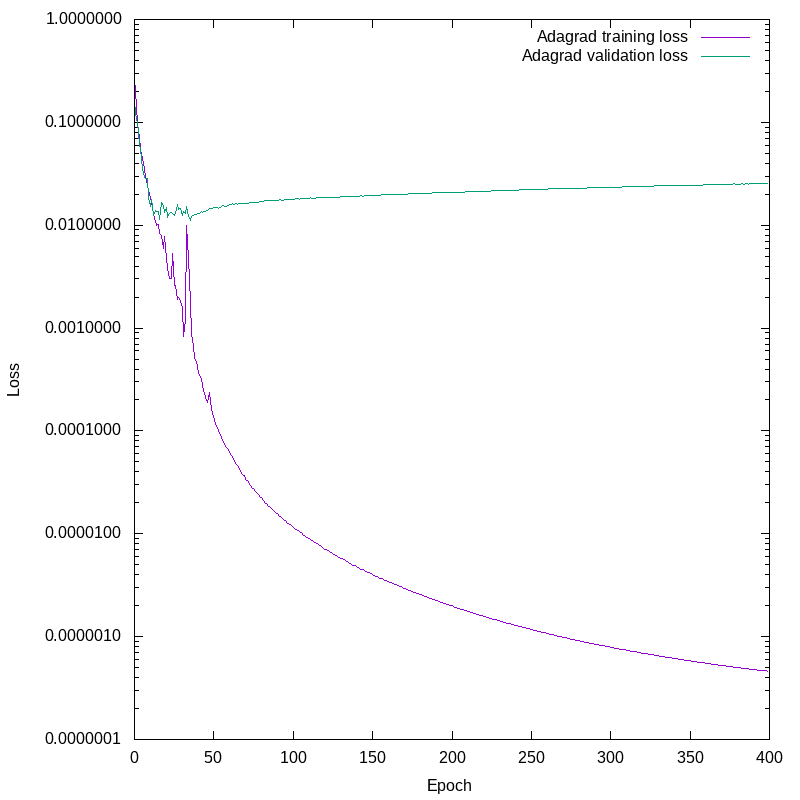
OK, I’m not going to turn this series of posts into a stack of plots of loss vs. epoch number, that’s not why we’re here. There is, however, one more I’d like to show. In the last post we saw some training results that were strongly suggestive of overfitting. I’m going to show one here that is unambiguous. This is the Adagrad optimizer in Keras, with default settings and batch size. This optimizer is a good choice for fitting sparse data. Even after thinning our dataset to remove many uninteresting inputs, any particular bit in the output set is still fairly sparse, so this seems a promising candidate.
Plotting the losses against epoch number again, we see this:
This is unambiguous. Note the logarithmic scale on the Y axis. Fairly early on, the validation loss detaches from the training loss. The network continues to improve the training loss by four decades, while the validation loss slowly increases. From about epoch 20 onward we are not improving the network’s ability to predict the future given new data, we are only getting it more and more obsessively correct about the training set, and our predictions on novel data are worsening.
All right, I’ve got four more optmizers bundled with Keras to test. I won’t post about those in detail unless something new appears, interesting in a different way. Once I’ve run through all the optimizers, I’ll present some other data about how well the resulting networks performed.
The index to the articles in this series is found here.
I was going to show the impacts of a few different modifications, but the first one showed some interesting effects that are worth discussing up front.
Knowlegeable readers who have been watching the source code carefully might have wondered at the use of the SGD optimizer in conjunction with a recurrent neural network. For such a network, the RMSprop optimizer is generally a better choice. I had the SGD optimizer there as a good initial baseline for comparison. I trained my network with that optimizer, with no regularizers, to show what happens as we start to tweak the settings.
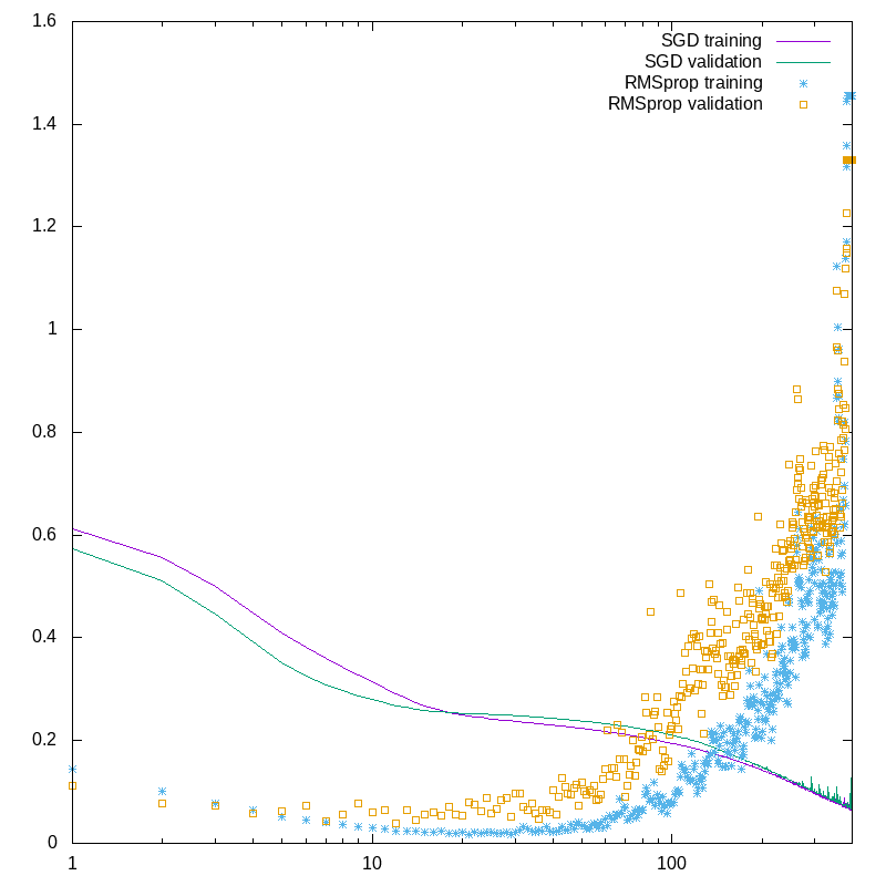
So, my first modification is to use the RMSprop optimizer. Running with the same data as we had for the SGD optimizer, we see something interesting. In first graph below, I plot the training loss and the validation loss for the SGD and RMSprop versions as we iterate through 400 epochs.
Figure 1
I’ve plotted the epoch number logarithmically to help show the detail in the early epochs.
First, look at the solid lines. The purple line is the training loss, the green line is the validation loss. They track together quite nicely, though there starts to be a bit of jittering of the validation loss at the higher epoch numbers.
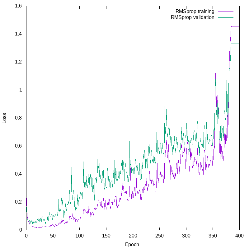
The RMSprop values are the points. Note that even after one generation, the loss is dramatically better than for SGD. There are two things we see in this plot. First, that fairly early on, the validation loss becomes much worse than the training loss. Second, that the training loss gets very bad after a while. Here’s another plot, with a linear X axis, showing just these two traces:
Figure 2
So, when the validation loss worsens even as the training loss improves, you have to think that we are probably overfitting the model. Overfitting is when the model becomes too finely tuned to the training data, and effectively becomes good at reproducing that specific dataset, rather than fitting to the trends that produced that dataset. The training and validation loss curves are also quite jittery (I avoid using the term “noisy”, as that has a precise statistical meaning). This overfitting doesn’t actually last long, because shortly afterward, the training falls apart.
The roughness of the loss curves can be traced back to the batch size. The fit() function in Keras still operates in batches. By default, it takes a batch of 32 inputs, runs them through the network, and generates a loss value. It then feeds this back into the network and tunes the weights. This process repeats with the next batch of 32 inputs, until the entire training set had been seen. Between epochs, the inputs are randomly shuffled, so the batches look different from one epoch to the next.
With its default settings, the RMSprop optimizer is quite aggressive. As each batch causes the network to be re-weighted, the variation between batches causes the weights to swing quite wildly. Just increasing the batch size reduces some of that early misbehaviour, because as the batches become larger they become statistically more alike, so outlier batches are less likely to appear and push the weights too strongly. In the case of my network here, with these default settings, we appear to have found a region of amplifying oscillations. Remember that loss is a measure of the amplitude of the departure of our model’s predictions from the true values. The oscillations in the weights are manifested as generally increasing loss values.
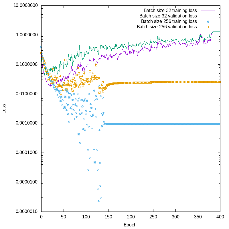
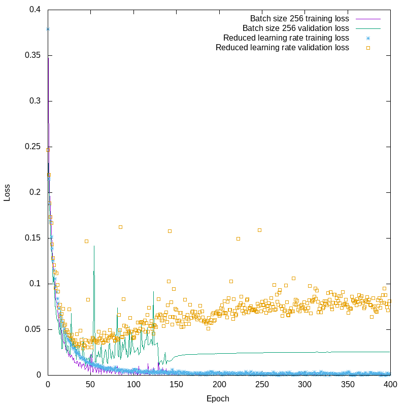
So, I said that the small batches, in conjunction with the aggressive weight tuning, were causing the oscillations. To demonstrate this, I re-ran the training, but using a batch_size of 256. Nothing else was changed. I plot the results here. This time I had to use a log scale in Y, just to be able to show the details of the differences, because of how far apart the loss curves are.
Figure 3
You can see that the amplifying oscillations have disappeared. Validation loss is still more than 10 times training loss with the larger batch size, so we have to worry about overfitting, but you can see that just before the training effectively stopped around epoch 170, the validation loss wasn’t monotonically increasing. The difference between the two losses might be purely statistical, due to differences between the training and validation datasets. There isn’t a clear fingerprint of overfitting.
Note at this point that we still haven’t started applying any regularizations. Those will come later.
OK, now you wonder if it might not be better to tune the learning rate than the batch size. There’s room for both approaches. For this particular project, a batch size of 32 really is too small, I’m training somewhat sparse binary data, so you want your batches large enough that they have a good chance of being representative, particularly when the training is as assertive as it is here with this optimizer.
So, what about the learning rate? The default value for the RMSprop learning rate in Keras is lr=0.001. For the next test, I reset the batch size to its default value of 32, and set the learning rate to 0.0001, reducing it tenfold. The following plot shows the difference between default learning rate and large batch size and lower learning rate with default batch size.
Figure 4
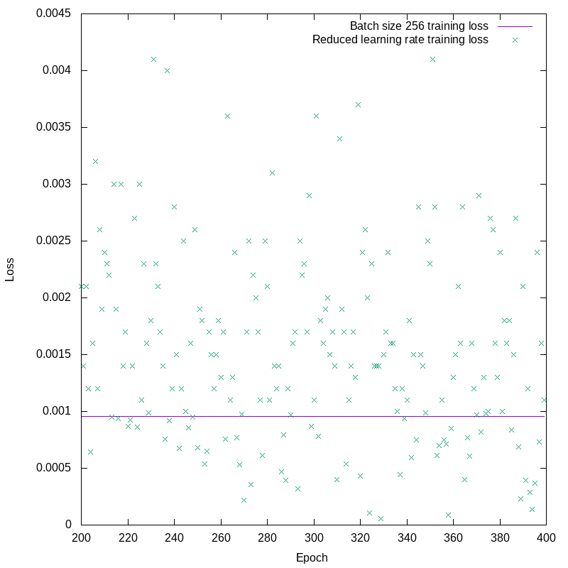
The training loss for the smaller learning rate looks, in this plot, to be quite similar to the larger batch size results. In fact, there’s a significant difference. Looking only at the training losses for epochs 200 and up, we see this:
Figure 5
The training loss, while relatively small, is still oscillating all over the place. The smaller learning rate has succeeded in suppressing the runaway oscillations, but it hasn’t changed the fact that there are oscillations. You’ll also notice in figure 4 that the training loss looks smooth on that scale, but the validation loss is all over the place. We’ve hit one of the issues I mentioned early on, unbalanced weights leading to undesirable sensitivity to the inputs. This is a kind of overfitting, and it’s what we plan to address when we finally reach the topic of regularization. In the mean time, though, we have concluded that the RMSprop optimizer really needs higher batch sizes when running on this particular project.
The index to the articles in this series is found here.
I’ve been talking about two datasets so far, training and validation. There’s a third dataset, holdout. This is data that the neural network never sees during training.
To review, here’s how the three datasets are used. The training dataset is run through the network to compute the loss, and that loss is used to adjust the weights, training the network.
The validation dataset is used, typically after each epoch, to compute a loss on data that the training never experienced. This is to help protect against overfitting. You can set up an early exit from the loop to stop training if the validation dataset starts to see worse results.
The holdout dataset is yet another dataset, one that was not seen either during training or validation. It’s there to see how well the trained network operates on new data.
Now, one thing about the holdout dataset is that it can be subsampled for different interesting behaviours. That is, you can remove entries that correspond to less interesting results. In our case, we’re going to focus on rain transitions. It’s not so impressive if the network predicts rain given that it’s raining right now, and similarly for predicting no rain if it’s not raining now. So, I filter the holdout dataset so that only entries where it rains in the future but isn’t raining now, or stops raining in the future but is raining now, are kept. These will form the basis for our evaluation of the network’s usability as we adjust parameters.
Another thing I’ve added to the training code is a hash of the training inputs and outputs. I’m going to be adjusting the network parameters and topology to try to find the best network I can, and I don’t want to discover later that I accidentally modified the input dataset, invalidating my comparisons. If the input set changes, the training will exit.
The index to the articles in this series is found here.
Finally, it seems we’re ready to start tuning this network. There will be several different approaches to try, and we’ll be examining the confusion matrix as we go.
The current training code is rptrainer2.py:
#! /usr/bin/python3

# Here we go again.  Training the neural network.

import rpreddtypes
import argparse
import random

import tensorflow as tf
# from tensorflow.keras.callbacks import TensorBoard, EarlyStopping

import keras
from keras.layers import Input, Dense, Concatenate, LSTM
from keras.models import Sequential, Model

import sys
import numpy as np


def getDataVectors(sequence_file, path_file):
    pathmap = {}
    seqmap = {}
    seqlist = []
    with open(path_file, 'r') as ifile:
        for record in ifile:
            fields = record.split()
            seqno = int(fields[0])
            pathmap[seqno] = fields[1]

    with open(sequence_file, 'r') as ifile:
        for record in ifile:
            fields = record.split()
            seqno = int(fields[0])
            seqmap[seqno] = list(map(int, fields[4:]))
            seqlist.append(seqno)

    random.shuffle(seqlist)

    # Need to load the size of the data samples by loading one data
    # file up front
    probeseqno = seqlist[0]
    probefilename = pathmap[seqno]
    reader = rpreddtypes.RpBinReader()
    reader.read(probefilename)
    rpbo = reader.getPreparedDataObject()
    datasize = rpbo.getDataLength()

    rvalX = np.empty([len(seqlist), 6, datasize])
    rvalY = np.empty([len(seqlist), 10])

    for index in range(len(seqlist)):
        base_seqno = seqlist[index]
        for timestep in range(6):
            ts_seqno = base_seqno + timestep
            ts_filename = pathmap[ts_seqno]
            reader = rpreddtypes.RpBinReader()
            reader.read(ts_filename)
            rpbo = reader.getPreparedDataObject()
            rvalX[index][timestep] = np.asarray(rpbo.getPreparedData()) / 255

        rvalY[index] = np.asarray(seqmap[base_seqno])

    return rvalX, rvalY, datasize


### Main code entry point here


lstm_module_nodes = 500
synth_layer_nodes = 300
num_outputs = 10


parser = argparse.ArgumentParser(description='Train the rain '
                                 'prediction network.')
parser.add_argument('--continue', dest='Continue',
                    action='store_true',
                    help='Whether to load a previous state and '
                    'continue training')
parser.add_argument('--pathfile', type=str, dest='pathfile',
                    required=True,
                    help='The file that maps sequence numbers to '
                    'the pathnames of the binary files.')
parser.add_argument('--training-set', type=str, dest='trainingset',
                    required=True,
                    help='The file containing the training set '
                    'to use.  A fraction will be retained for '
                    'validation.')
parser.add_argument('--savefile', type=str, dest='savefile',
                    help='The filename at which to save the '
                    'trained network parameters.  A suffix will be '
                    'applied to the name to avoid data '
                    'incompatibility.')
parser.add_argument('--validation-frac', type=float, dest='vFrac',
                    default = 0.2,
                    help = 'That fraction of the training set to '
                    'be set aside for validation rather than '
                    'training.')
parser.add_argument('--epochs', type=int, dest='nEpochs',
                    default = 100,
                    help = 'Set the number of epochs to train.')

args = parser.parse_args()


xvals = None
yvals = None
datasize = None

xvals, yvals, datasize = getDataVectors(args.trainingset, args.pathfile)


if args.Continue:
    if not args.savefile:
        print('You asked to continue by loading a previous state, '
              'but did not supply the savefile with the previous state.')
        sys.exit(1)

    mymodel = keras.models.load_model(args.savefile)

else:

    inputs1 = Input(batch_shape = (None, 6, datasize))

    time_layer = LSTM(lstm_module_nodes, stateful = False,
                      activation='relu')(inputs1)

    synth_layer = Dense(synth_layer_nodes, activation='relu')(time_layer)
    output_layer = Dense(num_outputs, activation='sigmoid')(synth_layer)

    mymodel = Model(inputs=[inputs1], outputs=[output_layer])

print('Compiling\n')
mymodel.compile(loss='binary_crossentropy', optimizer='sgd')
#                metrics=[tf.keras.metrics.FalsePositives(),
#                         tf.keras.metrics.FalseNegatives()])


# if args.savefile:
#     keras.callbacks.ModelCheckpoint(args.savefile, save_weights_only=False,
#                                     save_best_only = True,
#                                     monitor='val_loss',
#                                     verbose=1,
#                                     mode='auto', period=1)

print ('Training\n')
mymodel.fit(x = xvals, y = yvals, epochs = args.nEpochs, verbose=1,
            validation_split = args.vFrac, shuffle = True)


if args.savefile:
    print('Saving model\n')
    mymodel.save(args.savefile)
There is no generator, we’re using fit() now, as we can get all the training data into memory quite easily. I’ve concatenated the training and validation sets now, as I’m using the validation_split argument to fit().
I can regenerate a full set of intermediate binary files in under 2 hours using all of the cores on my machine, so we’ll be able to experiment with different module granularities as well, if needed, but that’s not going to be the first thing I look at.
I mentioned before that I’d be looking into using non-default weights, since I’m most interested in false negatives, so I want to emphasize reduction of that quantity in the training.
Network optimization isn’t usually a simple process. There are multiple parameters relevant to the training and topology, many of them interacting with one another. We’ll keep a record of attempts and outcomes, and see what works best for this specific project.
The index to the articles in this series is found here.
Well, over the course of the network design, we’ve gone from full precision inputs feeding modular neural networks up to LSTM, to 4×4 downscaled inputs feeding the same structure, to our current design, 800 total inputs per time step.
The effect of this has been to go from a system that took 2 days per epoch and overloaded my computer’s memory on batch sizes of 512 down to 2 hours per epoch, and then 90 seconds per epoch. I can also now fit the entire training set comfortably in memory.
Even with the speed improvements I put in with preprocessing the data, loading the entire set of data for one epoch took about 90 seconds. Suspiciously like the 90 seconds per epoch for running the system. Keras pre-loads the next batch of inputs in another thread so that the worker doesn’t have to wait for input, but if the worker is faster than the generator, it will still block. As we can now fit the entire dataset into memory, I modified the generator to cache the entire input set. This way it doesn’t have to go back to the disc between epochs. By not being disc-bound, we can get all cores on my box in use. I’ve got a 4-core machine.
With those further changes, resident space is about 2.5 GB per thread. Time per epoch is about 8 seconds. I’ll probably soon tear the generator out now that everything fits in memory. The current design actually keeps three entire copies of the training set in memory, and that’s silly. One copy is the cached data in the generator. One is the current data training the model, and the last is the preloaded data for the next batch.
The files are fairly minor variations of rpgenerator.py and rptrainer.py. Rather than reproducing them here, I just point you to their entries in the git archive. The files are in the top of the directory, named rpgenerator2.py and rptrainer2.py.
Well, now that we’ve got a system that trains nicely, it’s time to begin experimenting with settings. The first thing we’re going to want to do is to adjust the training parameters. That’s because I’m getting a loss improvement of about .0004 after each batch, regardless of batch size. So, when I train an entire epoch at once, I improve the loss by about 0.0004 in the early epochs, but if I divide the input set into 12 batches, I improve by about 0.005 per epoch. I’ve got to fix that.