The index to the articles in this series is found here.
While I continue to download training data from Environment Canada, I’ll talk a bit about this project.
So, I’ve been calling this a rain predictor. What is it, and what is it not? This neural network project aims to look at a time series of radar images, specifically 6 images taken at 10 minute intervals before the present. These images are taken from the Franktown radar facility SW of Ottawa and show only active precipitation. It then attempts to predict how these rain patterns will move through the region, and whether and when to expect rain in Ottawa. The radar images have a coverage with a radius of 240 km.
Rain that forms directly overhead has no radar warning, and this network will always be surprised by that. This code is limited to making predictions based only on a short (one hour) time series of active precipitation images. It will never pretend to know the weather next week, or tomorrow.
This isn’t a forecasting application, the scientists at Environment Canada have their own sophisticated models for estimating weather patterns over different parts of the country on a time scale of hours to days.
The obvious next question is, does it work with snow? The training data I’m downloading now is a continuous record (barring station outages due to hardware maintenance or failure). It will have training data from snow events when this is done. It so happens that the data I collected in 2015 and again in 2019 were all for summer months, so the network has not been trained against winter weather patterns. I should have enough data downloaded in about a week to train a new network, and I expect it will happily incorporate winter conditions.
I started this project thinking I could just throw the pixels from the radar into a neural network. I hadn’t quite appreciated the scale of that, and the resulting network was unusably slow to train. I then came up with a simple manual data convolution that allowed me to discard two levels of the neural network, and reduce each 480×480 .gif images to a record 800 bytes long. Six of these, less than 5k in total, is the entire input to the neural network for one prediction.
I tried various regularizations, activations, and topologies, but so far haven’t found any places for obvious improvement. Examining the distribution of weights with TensorBoard shows very good behaviour, no pathologies that produce unphysical dependencies on subsets of the data. I’m downloading more training data now, and once I’ve trained a new network from that I’ll check again to see if there’s anything I can do to improve it.
Training time on my home machine is about 20-30 minutes to get a stable, but overtrained network in 200 epochs with the training set I’ve been using until now. The best validation network can appear as soon as 5 minutes in.
The resulting network is at least as good as I am at reading the radar image sequence and estimating rain in Ottawa.
The index to the articles in this series is found here.
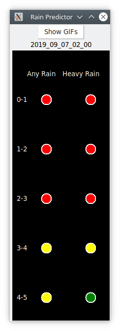
So, now that the network is doing as well or better than I can do looking at the same images, it’s time to present this data in a useful format. I decided a simple traffic-light style widget was simplest. Built using tkinter.
This is checked into the git tree under the name deskwidget.py. There’s also an associated configuration file, .rpwidget.conf.
This widget runs by watching the directory into which the downloading script puts its .gif files. When the collection script downloads a file, it also runs the make-rain-inputs.py script to generate the intermediate binary form. This widget polls that directory every second, and when it finds a new run of data files, it feeds them into the trained neural network and gets back confidence numbers for the 10 bits. These are then assigned colours. Green for confidence less than 0.05, red for confidence above 0.95, and yellow in between. A green light in a given time interval indicates that the network is confident that there will be no rain / no heavy rain in that interval. Red indicates that the network is predicting rain in that time interval. Yellow indicates uncertainty. These values are updated every 10 minutes, so an uncertain prediction might become certain a short time later. I can put this traffic signal up on the side of my screen, and then I can tell immediately whether or not to expect rain in the next 5 hours, and roughly when it might begin.
Here is a screenshot of the result:
This widget indicates that it is certain that it will be raining hard in the next 0-1 hours, 1-2 hours, and 2-3 hours. After that, it is uncertain whether or not there will be rain, but by 4-5 hours it is certain that even if there is rain, it won’t be heavy.
There’s also a button that pops up a window with the radar images from which these predictions were made, so that I can second-guess the network if I want to.
The time stamp is the UTC time on which this prediction is based. It should be less than 10 minutes old, but if the radar station goes down for maintenance there are no .gif files for download, and this widget will patiently hold steady until it obtains an hour of good data. The timestamp let’s me see whether the report I’m looking at is stale or not. I think I’ll highlight that, add code so that if the prediction is out of date, the timestamp has a yellow background.
The index to the articles in this series is found here.
I ran a few more experiments to try tweaks to the network configuration. I defined a measure of how well the network is performing on failed predictions. Essentially, the more the network was confident in a prediction that was incorrect, the larger the penalty. With a few obvious tweaks, I saw no marked improvement. Now, I didn’t run them a dozen times each to get statistics, but the results for all experiments are in a fairly narrow range anyway, I don’t think I’m going to see much improvement with these approaches.
The first experiment was to turn the activation function on the LSTM layer from ReLU to sigmoid. This is a good thing to try in any case, because ReLU is known to cause bad behaviour on recurrent layers, of which this is one. This didn’t result in any clear improvement on the failed-prediction measure.
Next, I switched the LSTM layer to tanh activation. Still no improvement.
Following this, I changed the activation on the synthesis layer from ReLU to Leaky ReLU. This is done by changing its activation to linear and then adding a LeakyReLU() layer above it. Still no improvement.
The last thing I tried was to make the network deeper, and add a second synthesis layer on top of the first. This also did not improve my measure any.
So, I’m going to leave refinement aside for now, and focus on collecting more training data and writing a little graphical widget that can sit on my desktop and give me a quick at-a-glance status of the network’s predictions. I think I’ll find that useful.
The index to the articles in this series is found here.
With a few tweaks to the phantom rain detection, suddenly things are looking much better. My two hour warning time is now 0.83, and the failed predictions are difficult cases. Examining the predictions that failed shows rain that forms directly overhead, with no warning on radar, or small rain pockets that could either pass by the city or pass overhead. They’re cases that I wouldn’t be able to predict better by looking at the same images. So, that’s a success. I can feed a set of radar images into the neural network and have it tell me whether or not to expect rain.
What’s left to do? Now we can still experiment a bit to see if we can find a way to reduce the fraction of failed predictions. Ideally we want incorrect predictions to have lower confidence than successful ones. By histogramming the (floating point) predicted values for successful and failed predictions, I hope I can come up with a confidence level. A value of less than 0.02 indicates a firm prediction of false. A value of greater than 0.98 indicates a firm prediction of true. In between, we have lower confidence warnings. There’s a cutoff at 0.5 between predicting positive or negative results. Shifting that cutoff has the effect of trading false negative for false positives, or vice versa. I’m not going to focus on this, though.
So, I’m going to try to play around with network settings now to see if I can separate the false positives from true positives, and conversely for negatives. Right now, there’s a handful of false negatives with a value less than 0.02, which indicates a firm false prediction. I’d like to train a network that minimizes those high confidence incorrect predictions.
Postings will probably slow down a bit now, as I experiment with settings and see how changes behave.
In the mean time, I’m happy with the results of this project.
The index to the articles in this series is found here.
I’ve now re-run the experiments over 200 epochs. In the first set of runs, the overfitting manifested fairly early, within 100 epochs, so I didn’t see a need to run out to 400 epochs this time. The SGD optimizer is still working at 200 (and was still working at 400 in earlier tests). The other optimizers have long since established their networks.
Experiment
Training Loss
Validation Loss
Two Hour Warning
SGD
0.3135
0.3057
0.00
RMSProp
0.0480
0.0796
0.82
Adagrad
0.0317
0.0823
0.78
Adadelta
0.0733
0.0829
0.77
Adam
0.0300
0.0872
0.77
Adamax
0.0340
0.1148
0.81
Nadam
0.0789
0.0929
0.80
Examining the loss numbers, it turns out that Adadelta hadn’t reached overfitting yet, and was still improving against the validation set, so I re-ran that one with 400 epochs, and it settled at a two hour warning fraction of 0.82.
One thing we see in this table is that there’s really no great difference, from a final model accuracy standpoint, between the various optimizers. Excluding the SGD, which would probably get there eventually if I let it run long enough, the other optimizers arrive at similarly accurate solutions. They differ in how quickly they arrive there, and as we saw in an earlier posting, some can diverge if the batch size is too small and the training is performed on batches that are not statistically similar to the overall population. Otherwise, I can limit my experimentation to a single optimizer, at least for a while. I might, at the end, re-run tests with all optimizers to see if any interesting differences in performance have been teased out by whatever configuration changes I make. I’ll be using the RMSprop optimizer for the next while, unless otherwise explicitly noted.
These numbers are disappointing, I liked it when they were at 0.96. Let’s analyse why the corrupted data did so much better, because it helps to emphasize why it’s critically important to have separate datasets for training and validation.
So, the problem occurred because I was manually shuffling two numpy arrays in parallel, using a Knuth shuffle. In this shuffling algorithm, we loop from the first element of the array to one before the last. At each element, we choose a random element between the element itself and the final element in the array, and swap this element with that other one. We never revisit earlier elements, and the random choice includes the same element, so there’s a chance that the element swaps with itself. It is easy to prove that in the final shuffled state, each element has an equal probability of being placed in each slot, so we have a true, fair shuffle.
I was swapping with the familiar mechanism: TMP = A; A = B; B = TMP. It appears, however, that the assignment to temporary space is a pointer, not a deep copy. So, modifying A also modifies TMP. This means that after the swap is complete, B appears twice, and A has disappeared. That assignment is a deep copy, if B is changed, A doesn’t change in sympathy.
Now, I was using Keras’ facility for splitting data into training and validation. This is done by taking a certain number of elements off the end of the input array before Keras does its own shuffling for purposes of splitting into batches.
We can analyse the effect of our broken shuffling on the distribution of elements, and, in particular, find out how many elements from the last 20% of the array wind up in the first 80% where the training will see them. Note that, because elements only move back in the array, training data never gets into the validation data, but validation data can wind up in the training data.
The probability that the first element in the training set will be copied from the validation data is
P_{1} = \frac{V}{N_{tot}}
where V is the number of elements in the validation segment, and N_{tot} is the total number of elements.
The probability that the second element will be copied from the validation data is
P_{2} = \frac{V}{N_{tot} - 1}
The expected number of validation elements that appear in the training data is, then
<N_{V}> = \sum_{k=0}^{N-V-1} \frac{V}{N - k}
This is just a bit of arithmetic on harmonic numbers.
<N_{V}> = V [ H_{N} - H_{N - k}]
This simplifies to:
<N_{V}> = V [ ln(N) - ln(N-k) + \mathcal{O}(\frac{k}{N(N-k)})]
When k is 20% of N, and N is in the thousands, as in our case, about 22% of the training set actually contains validation data.
So, unless your network has too few degrees of freedom to describe the problem, or is exactly balanced, then, barring convergence pathologies, you will eventually overfit the model. If your training data contains a significant fraction of your validation data, then you will appear to be doing very well on validation, because you trained against it.
What about the probability that any specific element in the validation set has not accidentally been placed in the training set? This is the product of the probabilities for each element in the training set:
Therefore, we expect 80% of our validation elements to be present in the training set, some duplicated, and 22% of our training set to contain validation elements. And that completely messes up our statistics, making it look like our network was doing much better than it truly was.
Where do we go from here? First, let’s look at the nature of a failing prediction. I pull one failure out and look at the historical rainfall, then the rain starting two hours later.
Historical data feeding network“Future” data feeding true Y vals 2 hours later
Yeah, there’s no rain there. What’s going on? The network got the correct answer, it’s the training “true” values that are wrong. You recall I had to deal with what I called “phantom rain”. That’s the scattering of light rain points around the radar station. Not really rain, it seems to be related to close range scattering from humid air. I don’t see a mention of this style of false image on Environment Canada’s page detailing common interpretation errors. I decided to use a rule that said that this false rain is declared to be occurring when only the lowest intensity of rain is seen within a certain radius of the radar station, and those rain pixels make up less than 50% of the area of the disc. Well, in the image that declares that there is rain in Ottawa at that particular time, there is a single phantom rain pixel of intensity 2, South-East of the station. This is enough for the data generation system to declare that another phantom rain pixel over Ottawa is real rain, and the training data gets an incorrect Y value. I brought up another image from a failed prediction, and there was a single pixel of intensity 3, North-North-West of the station.
All right, so my data cleaning operation didn’t work as well as it should have. Neural networks are notoriously sensitive to dirty data, as they work hard to imagine some sort of correlation between events that didn’t actually take place.
Recall that all of our networks overtrained, and based on the values of the training losses, reproduced their inputs essentially exactly when subject to a 0.5 mid-point decision cutoff between rain and no-rain. That means that our overtrained networks actually managed to declare those phantom rain pixels as rain, when they should not have done so. The best matching networks, though, the ones with the lowest validation losses, correctly indicated that there was no rain in those images, and we scored them lower because they failed to match the incorrect Y values. Validation loss doesn’t feed back into the network weights during training, so the network didn’t force itself to give wrong answers on these entries.
That’s actually very encouraging. Now all we have to do is to figure out how to identify phantom rain more accurately, regenerate our Y values, and try again. Well, I have a nice list of 30 or so bad cases, taken from the holdout data set. The neural network has helpfully presented me with a good set of incorrectly-classified images that I can use to improve my data cleaning efforts.
So, let’s not say we need exactly zero pixels of higher intensity than the lowest for the rain to be declared phantom rain. Instead, we’ll say that as long as there are fewer than 5 such pixels, there’s still a possibility of phantom rain. That’s an edit to prepare-true-vals.py.