The index to the articles in this series is found here.

Well, we’re about to start training the network, but it’s time to pause a bit and talk about our data. We will need training and validation data sets, for one. Confusingly, the keras documentation sometimes refers to the validation set as the test set, while common use does distinguish the two terms.

I’m going to take a short aside now to talk about another data set. I mentioned early on that this project doesn’t really make use of feature selection. Other projects, however, will. If you are performing feature selection before setting up your network, it turns out there’s a slightly subtle source of error that can creep in. If your feature selection is performed on your validation data you will introduce statistical biases. In effect, if feature selection identifies a feature that turns out to be a statistical anomaly, not a true feature of the data, then validating on that data set it will tend to reinforce the anomaly. If you keep the data sets separate, then the validation will not be weighted to support the anomaly, and you expect the measurements to revert to the mean.

OK, back to the rain predictor. So, I wrote a short script to split my data, called datasplit.py:

#! /usr/bin/python3

# Split the candidates file into training and validation sets.

import argparse
import random


parser = argparse.ArgumentParser(description='Split data into '
                                 'training and validation sets.')
parser.add_argument('--candidates', type=str, dest='inputfile',
                    required=True,
                    help='Path of the candidates file produced '
                    'by get-training-set.py')
parser.add_argument('--veto-set', type=str, dest='vetoset',
                    help='If supplied, its argument is the name '
                    'of a file containing candidates that '
                    'are to be skipped.')
parser.add_argument('--training-file', type=str, dest='trainingFile',
                    required=True,
                    help='The pathname into which training data '
                    'will be written.')
parser.add_argument('--validation-file', type=str, dest='validationFile',
                    required=True,
                    help='The pathname into which validation data '
                    'will be written.')
parser.add_argument('--validation-fraction', type=float,
                    dest='validationFrac', default=0.2,
                    help='The fraction of candidates that will be '
                    'reserved for validation.')
parser.add_argument('--validation-count', type=int,
                    dest='validationCount', default=0,
                    help='The number of candidates that will be '
                    'reserved for validation.  '
                    'Supersedes --validation-fraction.')

args = parser.parse_args()


vetoes = []

if args.vetoset:
    with open(args.vetoset, 'r') as ifile:
        for record in ifile:
            fields = record.split()
            vetolist.append(int(fields[0]))

validcandidates = []
trainingset = []
validationset = []

with open(args.inputfile, 'r') as ifile:
    for record in ifile:
        fields = record.split()
        if int(fields[0]) in vetoes:
            continue
        validcandidates.append(record)

random.shuffle(validcandidates)
numValid = len(validcandidates)
numReserved = 0

if args.validationCount == 0:
    numReserved = int(args.validationFrac * numValid)
else:
    numReserved = args.validationCount

with open(args.trainingFile, 'w') as ofile:
    trainingset = validcandidates[numReserved:]
    trainingset.sort()
    for line in trainingset:
        ofile.write('{}'.format(line))

with open(args.validationFile, 'w') as ofile:
    validationset = validcandidates[:numReserved]
    validationset.sort()
    for line in validationset:
        ofile.write('{}'.format(line))
    

This gets us our training set and our validation set. We take a random subset of the candidates out for validation, and keep the rest for training. I’ve chosen an 80% / 20% split because I don’t have such a very large amount of data yet. With a larger dataset, I’d keep a similar number of samples for validation, so the fraction used for validation would drop.

Now, I mentioned in an earlier article that I wanted to reduce the number of no-rain candidates, clear skies now giving clear skies later. I considered those uninteresting. Why didn’t I do the same for the converse case? Rain now means there will probably be rain 10 minutes from now. Well, I am interested in answering the question “if it’s raining now, when will it stop raining?” For that, I need those data elements.

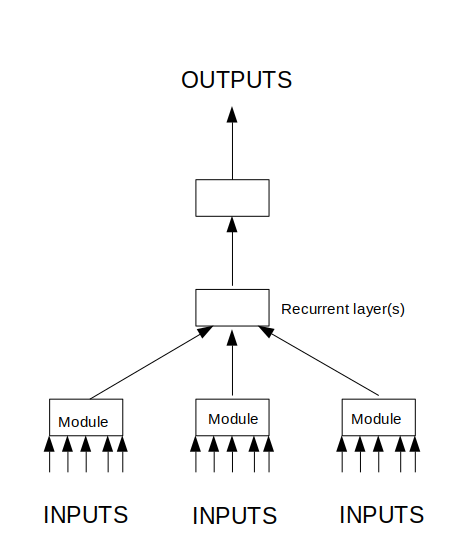
Next, our loss function. As the network trains, it has to establish an error metric that can be fed into the backpropagation step. I’ve got 10 independent binary fields. Well, not entirely independent, we never set the heavy rain bit when the rain-at-all bit is zero, but I’m going to ignore that subtlety for now. The loss function we want to use, then, is binary_crossentropy. We’re not looking for a one-hot solution, where only one bit is set. Next, though, we can talk about weights.

There are two measures that I’m really interested in, known as specificity and recall. Each is a fraction from 0 to 1. A high specificity indicates a low rate of false negatives, and a high recall indicates a low rate of false positives. I’m interested in high specificity, I’d rather be told it will rain, and then have it not rain, than go out thinking there wasn’t going to be rain, and getting soaked. So, by manipulating the weights, or by writing a custom loss method, I’m going to be trying to adjust the loss to favour specificity, even at a possible cost in lower recall.

The index to the articles in this series is found here.

OK, so we’re about to get to the actual writing of the program that will train our neural network. There are going to be many things going on there, and I wanted to start with a basic view of the network topology, with the accompanying Keras code.

Here’s a sample python program, keras-trial.py. It won’t be part of the final solution, but it demonstrates the way we’ll put pieces together in the rain predictor training code. I omit things like noise layers, pooling layers, and other modifiers that can be inlined trivially into this code.

#! /usr/bin/python3

# Figure out how to make our through-time siamese network with shared
# weights

import keras
from keras.layers import Input, Dense, Concatenate, LSTM
from keras.models import Sequential, Model

import sys
import numpy as np


ring0_pixels = 5
ring1_pixels = 4
timesteps = 2
batch_size = 128
ring0_module_nodes_0 = 4
ring0_module_nodes_1 = 3
ring1_module_nodes_0 = 4
ring1_module_nodes_1 = 3
synth_layer_nodes = 3
num_outputs = 3




ring00 = Input(batch_shape=(batch_size, timesteps, ring0_pixels))
ring01 = Input(batch_shape=(batch_size, timesteps, ring0_pixels))
ring10 = Input(batch_shape=(batch_size, timesteps, ring1_pixels))
ring11 = Input(batch_shape=(batch_size, timesteps, ring1_pixels))

ring0_model = Sequential()
ring0_model.add(Dense(ring0_module_nodes_0))
ring0_model.add(Dense(ring0_module_nodes_1))

ring1_model = Sequential()
ring1_model.add(Dense(ring1_module_nodes_0))
ring1_model.add(Dense(ring1_module_nodes_1))

scanned00 = ring0_model(ring00)
scanned01 = ring0_model(ring01)
scanned10 = ring1_model(ring10)
scanned11 = ring1_model(ring11)


aggregated = Concatenate()([scanned00, scanned01, scanned10, scanned11])


time_layer = LSTM(3, stateful=False, return_sequences=True)(aggregated)

synth_layer = Dense(synth_layer_nodes)(time_layer)
output_layer = Dense(num_outputs)(synth_layer)

model = Model(inputs=[ring00, ring01,
                      ring10, ring11],
              outputs=[output_layer])
# model.compile(optimizer='SGD', loss=keras.losses.mean_squared_error)

I wanted to show that I can have multiple neural networks, each operating independently on multiple partitions of the input data, these modules then feed up into a recurrent network, on to an interpretation layer, and output.

For simplicity in this demo implementation, I’ve divided my input data into four partitions, ring00, ring01, ring10, and ring11. I create a two-layer dense neural network called ring0_model that acts separately on ring00 and ring01, and a second two-layer dense neural network, ring1_model, that acts on ring10, and ring11. The four output tensors of these two models are then concatenated into a list of values which feed into the recurrent LSTM layer. This produces a set of outputs that are processed by a dense hidden layer, and then an output layer.

In reality, I’ll have 34 different rings feeding 10 different models. Each of those 10 models will produce some number of outputs that are passed to the LSTM layer for through-time analysis, then on to the synthesis layers for output. There will be 6 time steps passed through LSTM before output is collected for error estimation.

The batch_size is a count of the number of training candidates that will be passed through the network before back-propagation and weight updating occurs. This may be smaller than the total number of training candidates, so there will be multiple weight updates over the course of completing a single pass through the training data (called an epoch).

And there we have the bare bones of our Keras implementation. Next, we write the actual code that feeds image data into the network, and start experimenting with settings and parameters.

UPDATE #1 (2019-08-23): Included a link to an index of articles in this series.

The index to the articles in this series is found here.

I’ve been throwing about a lot of somewhat technical terms, and it occurs to me that I probably should have spent some time explaining them up front.

If your understanding of neural networks is along the lines of saying “a directed graph in layers, with neurons that sum their inputs in a linear combination, add a bias, and feed through a sigmoid function before going to the next layer”, that’s a start, but there’s much more subtlety than that once you get into the details.

Some types of layers:

I’ve mentioned various types of layers before. Note, however, that a neural network can be made without layers at all, though doing so poses its own difficulties of mathematics and implementation.

The simplest layer people usually think of in the context of neural networks is the dense, or fully connected layer. Such a layer might have N inputs, and consist of M neurons. Each neuron will take, as input, all of the N inputs and produce a single output. The topology is symmetric, from a connection standpoint all of the neurons look equivalent. Of course, as the layer is trained, weights will change, and the neurons will not behave identically. From an ease of implementation standpoint, one usually treats the bias term as an additional input, with its value set to 1. This means that each neuron has N+1 weights, and there are M neurons, for a total of M*(N+1) weights. In implementation, these will generally be stored in a tensor. Think of a tensor as an array with an arbitrary number of dimensions.

I’ve mentioned convolutional layers a few times in this series. This is a layer that acts on groups of proximate data. The simplest way to think of a convolutional layer is to imagine a system for computer vision. The inputs are separate pixels in the image laid out on a two-dimensional grid, and we can describe certain pixels as being adjacent to certain other pixels. We can construct a neighbour graph that states that the pixel at (10,9) is adjacent to the pixel at (10,8). A convolutional layer, rather than taking the values of the pixels as inputs, performs a convolution operation on the pixels. For each pixel it produces one or more values that are functions of the pixel and its neighbours. If you think of the values on the pixels as representing a function in two dimensions, then the convolution is a function of the function. There are several different convolutions one could apply, including nonlinear ones that involve min() and max(), but a simple linear one would be this: imagine that you want to use only the eight nearest neighbours in a square grid, then you have the centre pixel and the eight pixels that surround it, for a 3×3 grid of pixels with their associated values. The convolution function itself is another 3×3 grid of numbers. The convolution operation is to multiple these two matrices together, then add the values of the resulting 3×3 product matrix together to produce a single number. The convolution operation then slides over to a new next pixel and the operation repeats. There is a lot more behind convolutional layers, but I’m not going to do a thorough discussion of them here. You might want to imagine a one-dimensional problem, say a noisy signal on a measurement, and an associated kernel that looks like [0.2,0.2,0.2,0.2,0.2], and what this convolution would do to the signal.

A sparse layer is the converse of a dense one. It’s a layer in which not all neurons receive all inputs. One typically generates these topologies by hand, due to some specific knowledge of the problem space, though there are automated techniques, such as training a dense network for a while and then forcefully cutting low-weight inputs to zero. The aim here is to reduce computational effort by removing connections that have little bearing on the final answer. There have been reports, however, that these layers yield networks that are prone to convergence problems, so one should bear that possibility in mind when using sparse layers.

A recurrent layer is one that feeds back into itself. That is, its inputs at time N+1 include one or more values derived from a function of its outputs from one or more earlier timesteps. The details of this function lead to different types of recurrent networks, including simple, GRU, and LSTM. A recurrent neural network is one way in which the network can be designed to track behaviour through time, which is exactly what I’m trying to do in the rain predictor.

These four cases make a good introduction to the kinds of active layers that are often used in neural network problems. I’m not including layers that Keras and TensorFlow define but which I think of more as topological transformations, such as pooling or merge layers, or simple functional layers where each neuron takes a single input, applies a mathematical operation on that one value (such as computing its square or adding noise) and produces a new value.

Activation functions

Without a nonlinear activation function, the outputs of a neural network are a simple linear combination of inputs (including bias), which means it can be represented by a single matrix, so the layers could be collapsed into a single layer. To get interesting behaviour, you need a nonlinear activation function. This is the function that is applied to the linear combination of inputs to produce the output.

Keras supplies several activation functions, the choice of function is a bit subtle. Typically one doesn’t use sigmoid or tanh activation functions on the intermediate layers because it’s easy to find oneself in the regime of small but non-zero derivatives that cause significant slowdowns in the training process, as it depends on gradient descent. Common choices for the intermediate layers are ReLU, leaky ReLU, and hard sigmoid, all of which have bounded derivatives that exclude small non-zero values.

For our output layer, we will be using sigmoid functions, since we’re looking for a 0/1 distinction, and sigmoid is the obvious candidate.

Regularization

There are some common problems that can arise in neural networks. Regularization can help address at least two big ones: overfitting and unrealistic high weights on certain inputs.

Overfitting is a common concern. It’s one reason I’ve spent so much effort on minimizing neurons in our neural network. With enough parameters in play, you can run a line through any collection of points. A neural network might become obsessively accurate at reproducing the training data, at the expense of generality. This is what is generally referred to as overfitting. We will address this concern statistically in a later posting.

The other common problem is an unrealistically high dependence on a particular input. The neural network might sniff out some coincidental correlation between some subset of the inputs and the desired outputs, and put a lot of weight on that. This is, in effect, another manifestation of overfitting, but stands a bit in its own category.

Regularization is how one typically avoid overfitting. A first obvious technique is referred to as “early stopping”. As you continue to train, your network becomes better at matching the training data. It may, however, start to drift ever further from your validation data (you will have validation data). Early stopping just asserts that once the network’s performance on the test data starts to degrade, that you stop your training. Naturally, it’s not quite that simple, the agreement with the validation data can worsen before ultimately improving further, so various heuristics are used to decide when to stop training.

Some other regularization techniques rely on the observation that neural networks are, or should be, fairly robust in the face of neuron dropouts or noisy data. You train the network while it is faced with problems like the deletion of a significant fraction of its nodes. Between training passes, the nodes that are deleted change. This prevents any small set of nodes from dominating the behaviour of the system, because if some of those nodes are deleted, the network will suddenly perform poorly, and will train away from that configuration.

One can also introduce noise in the outputs of one layer, as inputs to the next. This helps to force the network to configure itself for a broader volume of the phase space of inputs, thereby becoming more general, and less likely to overfit.

Finally, to avoid the problem of extremely large coefficients in some places in the network, a penalty term can be applied in the error estimation simply due to the presence of large coefficients. This causes the network to push itself away from configurations that have large coefficients.

One regularization technique that is sometimes applied is to delete weights that are small but non-zero, and set them to zero. This is helpful for reducing network complexity, but, as noted above, it is suggested that convergence suffers if this is applied too liberally.

In conclusion

So, that’s a brief overview of some of the terms I’ve been throwing around in this set of articles. One can practically write an entire book around the content of each paragraph above, so there’s a lot more detail to explore.

UPDATE #1 (2019-08-23): Included a link to an index of articles in this series.

The index to the articles in this series is found here.

Machine learning is, as they say, a very active field. There are many ways we can go from here, and we’re likely to try a few different approaches as we explore this problem.

Now, as I’ve alluded to in previous articles, my initial thought is to make this a modular neural network. Divide the input space into separate modules that are then processed, rather than producing a network that cares intimately about the details of individual pixels. Rain far away is probably not as interesting as rain close to Ottawa, so we can use bigger buckets of points far away. I described a dartboard-like module layout. Here’s an example of what I’m thinking might work:

Here, the radar station is at the red star, and Ottawa is roughly on the green spot. This divides the pictures into 33 clusters.

I’d also like to add another module. I’ll call this a tripwire. It will process a ring of pixels around Ottawa, at a distance of, say, 30 pixels. Our graphs have a resolution of one kilometre per pixel, so this represents a sensitive region extending roughly an hour out of Ottawa, for moderate wind speeds. If rain starts falling in this tripwire, there’s a good chance that rain is imminent in Ottawa, and I want my neural network to pay particular attention to this condition.

These modules will do some analysis of the pixels they contain, and then will produce a set of outputs. We haven’t decided yet how many numbers will be output, we’ll experiment a bit later.

So, that’s a logical description of the layout, now to details. I’m expecting each module to involve a dense neural network of two layers. I’m not planning to make them convolutional to begin with, but might try that later, as convolutional layers might be able to distinguish incoming cold fronts, where a line of rain crosses the Ottawa Valley. In an earlier posting I dismissed the idea of using convolutional layers, but on further consideration, I’m not going to rule it out now.

Now, what about independence? Might it be possible to use a single network to process all modules in the outer ring, another for the ring inward of that, and so on? This would reduce the number of weights in our model almost eight-fold, and might therefore make the problem more tractable in terms of training time and memory consumption. This is tempting, but remember the issue with transformations that aren’t part of the symmetry group of the square grid. We have D_2 and D_4 symmetry groups available, which means that we can do rotations of 90 degrees without loss, but 45 degree rotations are a bit tricky, we lose the guarantee of 1-1 mapping, and we can’t ensure that all modules have exactly the same number of pixels in them. So, a compromise, we’ll use two independent networks per ring. Two adjacent modules will have independent neural networks, and then rotations of 90 degrees will span the entire ring. We can build a mapping of pixels to modules that guarantees identical geometries and numbers of pixels, preserving neighbour relationships.

Above these modules, I expect to have at least two more dense layers that process the inputs from the modules and compute the outputs. These layers will be relatively light-weight. If each module produces 5 outputs, and we have 34 modules, then we’ve got about 170 inputs to the synthesis layers at the top.

And, what about time dependence? I’m not thinking of using embedding at this time, where we treat the time dimension as just one more spatial dimension and so wind up with six times as many inputs and six times as many weights. I don’t really think that the output at time T+1 depends on subtle calculations of the input at pixel P1 at time T-3 and also pixel P2 at time T-1 and pixel P3 at time T, so having all that data on hand and feeding into the same network simultaneously seems undesirable.

The way I’m planning to handle the time series is with recurrent layers. I’m thinking GRU or LSTM layers, rather than simple recurrent neural network layers. My initial thought was that the recurrence would be in the modules, but I’ve changed my mind. The problem we’re trying to solve isn’t best described by the time evolution within a module (geometric sector), but the time evolution of movement between modules. So, the recurrent layer(s) would be in the synthesis layers above the modules.

Here’s a layout of the flow of data in this topology. The arrows indicate flow of information, not single values. Images are fed into the modules, and some analysis is done. The modules produce some information which is fed into one or more recurrent layers whose job it is to analyse the time-dependent behaviour of the system. This then feeds into one or more layers that roll everything up into our rain predictions.

So, what I’m imagining the network is probably going to do when it has trained is that the modules will produce some sort of proxies for rain intensity, radial movement, and tangential movement of rain structures. The layer(s) above will tie together this information from different geometric sectors through time, along with the tripwire module, to produce some outputs that are related to how rain is moving through the system. The top layer(s) then produce the outputs.

In the next posting, I plan to review some terminology and approaches, for those who are not yet familiar with the details of neural network programming.

UPDATE #1 (2019-08-23): Included a link to an index of articles in this series.